The Dynamics of Learning
In the post on spectral learning, we saw that a loss function alone does not determine what gets learned. The optimizer matters too, and its implicit bias affects generalization at first order. In the post on the neural tangent kernel, we saw that gradient descent on a network reduces to two coupled equations: one governing how errors evolve, and another governing which errors interact.
Both points illustrate that learning algorithm is a dynamical system, and loss minimization is only one way to specify its dynamics. Some well-known algorithms came from the other direction. AdaBoost, for example, was introduced as a reweighting rule before it was understood as descent on an exponential loss.
That suggests a different program: write down the dynamics you want from first principles, then prove that they are stable and converge. This is far less standard than minimizing a loss, but it may be closer to how biological systems learn. In practice it is hard: convergence has to be established case by case, and many sensible rules turn out to be optimization in disguise.
This post collects what I learned along the way. It has three goals:
- Characterize the implicit bias of a learning rule concretely, through the quantities it conserves.
- Show that these biases need not be designed into the optimizer: an architecture can build them.
- Give a family of dynamics that is not gradient descent on any loss, still converges, and has a slot for importing other biases.
The setup
The setup is again a linear model. Given data $X$ and $y$, we estimate $y$ by $Xw$ with squared loss
\[L(w)=\tfrac12\|Xw-y\|^2.\]Write the residual as $e=Xw-y$, the gradient as $g=\nabla L(w)=X^\top e$. Now imagine writing the learning rule from scratch. A useful template is
\[\dot w=-MX^\top r.\]Here $r$ is an error state that determines how examples exert pressure on the parameters, while $M$ determines the geometry and how errors communicate. Ordinary gradient flow is the simplest case: $r=e$ and $M=I$. In the context of optimization, $M$ is just a preconditioner. You can generate a huge variety of learning methods in this framework (including different loss functions), especially once you add dynamics to $M$ and $r$. This note is in continuous time for simplicity.
Invariants
When the loss has multiple minimizers, invariants of the dynamics can determine which one is selected. An invariant is a function $Q$ whose value remains constant along the trajectory:
\[\frac{d}{dt}Q(w(t))=0.\]The trajectory is therefore confined to the level set ${w:Q(w)=Q(w_0)}$ determined by its initialization. Suppose the flow converges to a minimizer $w_\infty$ of $L$. This has to be checked rule by rule, and holds for the descent-type examples below.1 By continuity, $Q(w_\infty)=Q(w_0)$, so
\[w_\infty\in\arg\min L\ \cap\ \{Q=Q(w_0)\}.\]The loss supplies the first set; the dynamics supply the second. When the minimizer is unique, the invariant has no choice to make. But in least squares the minimizers can form an affine set $w^\star+\ker X$—a set of interpolants when the data are realizable—and the loss has nothing further to say. If the invariant supplies enough independent constraints along $\ker X$, its level set can intersect the minimizer set at a single point.
When Invariants are Regularizers
When $M$ is the inverse Hessian of a strictly convex function $R$, e.g. $\dot w=-\nabla^2R(w)^{-1}g,$ the invariant has a particularly satisfying interpretation. Since $\frac{d}{dt}\nabla R(w)=-g$, the dynamics are gradient flow in the mirror coordinates $\nabla R(w)$. Because $g$ always lies in the row space of $X$, its null-space component never changes: $Q=P_N\nabla R(w)$ is conserved, where $P_N$ projects onto $\ker X$. This invariant is exactly the optimality condition for a regularized problem. The flow converges to
\[w_\infty=\arg\min_{w\in\arg\min L} \left[R(w)-R(w_0)-\nabla R(w_0)^\top(w-w_0)\right],\]the minimizer closest to its initialization in the geometry induced by $R$ (Gunasekar et al., 2018). In this case, the invariant is the implicit regularizer.
Ordinary gradient flow takes $R(w)=\tfrac12|w|^2$, recovering the familiar minimum-norm solution. For adaptive methods such as RMSProp and Adam, the preconditioner depends on gradient history rather than on $w$ alone, so their implicit bias is much harder to characterize this way.
Biases from Architectures
In this section we’ll see that by changing the parameterization/architecture of the linear model we can generate $M$, e.g. a learned geometry. Let $w=W_2u$, with $u\in\mathbb R^k$ and $W_2\in\mathbb R^{d\times k}$, and run gradient flow on the factors. The predictor only sees their product, but the optimizer moves them separately. Eliminating the factors gives
\[\dot w=-Mg,\qquad M=\|u\|^2I+W_2W_2^\top,\]where $M$ is positive semidefinite. More strikingly, the effective dynamics close:2
\[\begin{aligned} \dot w &= -Mg,\\ \dot M &= -2(w^\top g)I-gw^\top-wg^\top. \end{aligned}\]Everything the factorization contributes is therefore captured by
\[w(0)=W_2(0)u(0),\qquad M(0)=\|u(0)\|^2I+W_2(0)W_2(0)^\top.\]After initialization, the factors can be discarded: the predictor follows a closed adaptive-preconditioning system in $(w,M)$. Two networks can represent the same $w(0)$ but induce different $M(0)$, and hence different effective optimizers. The architecture has constructed optimizer-like dynamics on the effective parameters—the usual observation that depth acts as a preconditioner (Arora et al., 2018), viewed from the other side.3
Further constraints on the architecture let us deduce a more explicit prior. Let $w=u\odot v$. The flow conserves $c_i=u_i^2-v_i^2$, while its effective preconditioner is
\[M=\operatorname{diag}(p_i(w_i)),\qquad p_i(w_i)=\sqrt{c_i^2+4w_i^2}.\]Because each $p_i$ depends only on $w_i$, this is an inverse Hessian with $R_i’‘=1/p_i$. Small coordinates begin stiff and become more plastic as they grow. Starting from $w_0=0$, $u=\alpha\mathbf 1$, and $v=0$, the resulting potential approaches an $\ell_1$-type geometry as $\alpha\to0$ (Woodworth et al., 2020). While no explicit sparsity term appears in the loss, the system architecture provides it implicitly.
An Optimizer Sidecar
Write an effective rule as $\dot w=-Ag$ and decompose $A$ into a symmetric part $G$ and a skew part $S$. Only the symmetric part affects the loss:
\[\dot L=-g^\top Gg,\qquad g^\top Sg=0.\]Every rule so far, including those built by the architecture, lives in $G$: descent on the loss in some geometry. The skew part is invisible to the instantaneous loss derivative. It can therefore steer the trajectory without directly opposing descent.
This gives another way to introduce a preference. Weight decay modifies the objective, so its shrinkage competes with fitting the data. Instead, take a shrinkage direction $h$ and keep only its component orthogonal to the gradient:
\[\dot w=-(I+\lambda S)g,\qquad S=hg^\top-gh^\top.\]I will call the extra term circulation. Since $S$ is skew, $\dot L=-|g|^2$ exactly as for gradient flow at the same point, while the extra motion vanishes as $g\to0$. In general this vector field is not the gradient of any modified loss: the preference lives in the dynamics.
For that preference, take
\[h(w)=\tanh(w/\tau)=\nabla R_\tau(w),\qquad R_\tau(w)=\tau\sum_i\log\cosh(w_i/\tau).\]Near zero, $h$ behaves like weight decay; for large coordinates it approaches $\operatorname{sign}(w)$, pushing coordinates toward zero with roughly equal force. Because this map is nonlinear, $h(w)$ can have a component in $\ker X$ even when $w$ lies in the row space. Circulation can therefore move the endpoint away from the minimum-norm solution without changing the loss-dissipation identity.4
The smallest example that can be drawn has two examples and three parameters, so the solutions form a line. Starting from $w_0=0$ with $\tau=0.1$ and $\lambda=1$, gradient flow remains in the row space. Circulation instead accumulates a null-space component while $|g|$ is large, which freezes at $n^\top w=0.24$ as the gradient vanishes. Both converge to the solution line, but at different points.
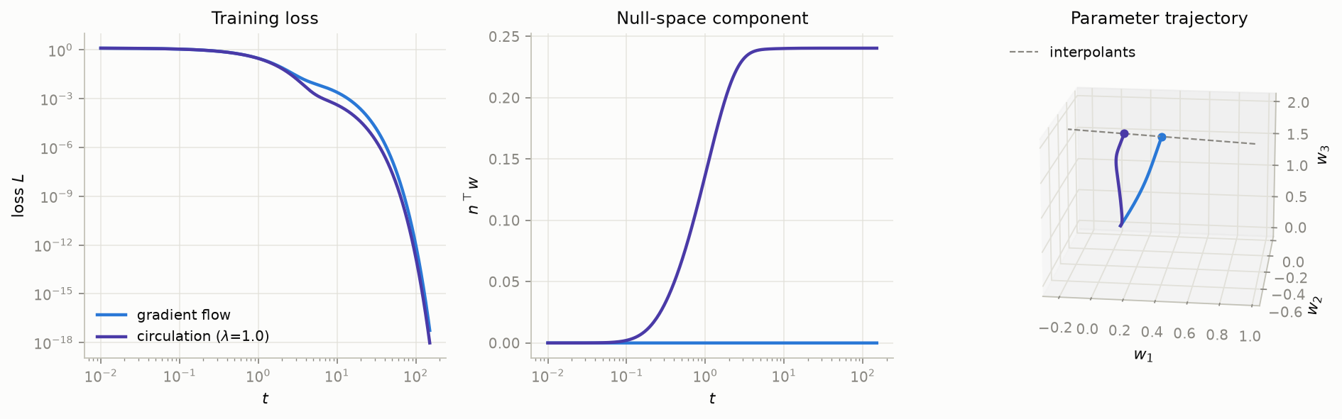 Both methods converge, but to different solutions. Left: training loss. Middle: motion along the unit null vector $n$; gradient flow remains at zero while circulation accumulates a null-space component. Right: the trajectories end at different points on the line of interpolants (dashed). The loss curves need not coincide: both satisfy $\dot L=-|g|^2$, but they encounter different gradients along different trajectories.
Whether the new endpoint is any better is another question. In this example circulation lowers $R_\tau$ from $2.47$ to $2.30$ while slightly increasing $|w|$, from $1.959$ to $1.974$. Nothing here implies that the resulting solution generalizes better.
Creating Sane Dynamics is Hard
A sensible verbal rule can hide a bad dynamical system. For example, let errors accumulate:
\[\dot r=e,\qquad \dot w=-X^\top r.\]If an error persists, keep building pressure until it is corrected. This is the integral term of a PID controller, and it sounds appealing: unlike gradient flow, the system remembers past errors. But differentiating gives $\ddot e=-XX^\top e$. The reachable residual modes are undamped oscillators, while any irreducible residual persists. Generically, the system does not converge.
In fact, these dynamics are descent–ascent on $r^\top(Xw-y)$, with $r$ acting as a Lagrange multiplier enforcing $Xw=y$ exactly. The rule I thought I was writing was about accumulated pressure. The rule I actually wrote was a hard constraint. The repair is one term: $\dot r=e-r$. Adding this leak turns the oscillator into damped least-squares dynamics. Nothing in the verbal rule predicts the oscillator. That is what makes dynamics-first design hard: plausible local rules can have unexpected global behavior, and the convergence guarantee supplied by descent on an objective is not a formality.
Final Thoughts
It is hard to get away from framing learning as a loss plus an optimizer, and for good reasons. Descent on an objective gives you convergence almost for free, and losses like maximum likelihood come with statistical justification. The integral rule shows what you lose without that guarantee: a sensible rule turned out to be an undamped oscillator.
But it is not the only way to build a learner that converges. A factorized network builds its own adaptive preconditioner, and its bias comes from the parameterization and initialization rather than from anything written into the objective. Circulation goes further. The skew term changes where the flow lands without touching the rate of descent, so any preference you can express as a direction $h$ comes along without costing convergence.
What I was really after is a template: a way to write down learning dynamics without re-proving convergence and stability each time. Neural architectures are one template. The kernel $JJ^\top$ is positive semidefinite by construction, so gradient flow through any architecture descends the loss. The split $\dot w=-(G+S)g$ is another: the loss descends at a rate set by $G$ alone, and the skew part $S$ is free to carry other preferences. Inside a template, the design work moves to what I actually care about, local rules for how errors compete and evolve, with invariants that encode the priors. That is closer to a physics of learning than to a choice of model.
Gunasekar, Suriya, Jason Lee, Daniel Soudry, and Nathan Srebro. “Characterizing Implicit Bias in Terms of Optimization Geometry.” ICML, 2018.
Arora, Sanjeev, Nadav Cohen, and Elad Hazan. “On the Optimization of Deep Networks: Implicit Acceleration by Overparameterization.” ICML, 2018.
Woodworth, Blake, Suriya Gunasekar, Jason Lee, Edward Moroshko, Pedro Savarese, Itay Golan, Daniel Soudry, and Nathan Srebro. “Kernel and Rich Regimes in Overparametrized Models.” COLT, 2020.
Appendix
A. Convergence of the circulation flow
Let $h$ be bounded and locally Lipschitz. The vector field in the body is locally Lipschitz, and $\dot L=-|g|^2$ gives
\[\int_0^\infty\|g(t)\|^2\,dt<\infty.\]Decompose $w=u+z$ into its row-space and null-space components. The loss sublevel set bounds $u$, while
\[\dot z=-\lambda\|g\|^2P_Nh(w)\]has finite total variation because $h$ is bounded. Thus $z$ converges, $w$ remains bounded, and the local solution extends for all time. Boundedness also makes $\dot g=X^\top X\dot w$ bounded, so $g$ is uniformly continuous. Together with the finite integral above, this gives $g(t)\to0$. The row-space component therefore converges to the unique row-space least-squares solution $X^\dagger y$, while the null-space component converges to
\[P_Nw_\infty=P_Nw_0-\lambda\int_0^\infty\|g(t)\|^2P_Nh(w(t))\,dt.\]If the data are realizable, $w_\infty$ is an interpolant. Coordinatewise $h(w)=\tanh(w/\tau)$ is bounded and globally Lipschitz.
-
The factorized model below has exceptional initializations—for example $u=0$, $W_2=0$—where the induced preconditioner vanishes and the flow can stop at a non-minimizer. ↩
-
From $\dot u=-W_2^\top g$ and $\dot W_2=-gu^\top$: $\dot w=-(|u|^2I+W_2W_2^\top)g$, $\tfrac{d}{dt}|u|^2=-2w^\top g$, and $\tfrac{d}{dt}W_2W_2^\top=-gw^\top-wg^\top$. ↩
-
The factor dynamics also preserve $W_2^\top W_2-uu^\top$. This constrains the representation across layers but is not needed to evolve the reduced system once $(w(0),M(0))$ is known. ↩
-
For linear least squares, boundedness and local Lipschitz continuity of $h$ are enough to make the flow global and convergent to a least-squares solution; coordinatewise $\tanh(w/\tau)$ satisfies both conditions. Appendix A gives the argument. ↩