Much of linear least-squares learning is spectral filtering
In the last post I noted that OLS, Ridge, and PCR can all be written as spectral methods. It turns out gradient-based methods fit the same mold as do most of their variants (learning-rate schedules, momentum, early stopping). Rather than a zoo of special cases, there is one common framework based on a choice of filter function $g$. The right choice of $g$ boils down to the spectrum of your data and where the signal sits along it.
The spectral zoo
Take the linear model $y = X\beta^\star + \varepsilon$, with $\mathbb{E}[\varepsilon] = 0$, $\operatorname{Cov}(\varepsilon) = \sigma_\varepsilon^2 I$, and the thin SVD
\[X = U\Sigma V^\top, \qquad \Sigma = \operatorname{diag}(\sigma_1, \dots, \sigma_r), \quad \sigma_1 \ge \dots \ge \sigma_r > 0.\]Every method below produces fitted values of the form
\[\hat y = U\, g(\Sigma^2)\, U^\top y = \sum_i g(\sigma_i^2)\,(u_i^\top y)\, u_i,\]where $g(\Sigma^2) = \operatorname{diag}(g(\sigma_1^2), \dots, g(\sigma_r^2))$. The estimator is entirely determined by the scalar filter $g$: it says how much of the data’s component along each direction $u_i$ survives into the fit. OLS is a projection which keeps everything, which is to say $\hat y = UU^\top y$, e.g. $g \equiv 1$.
Here is the zoo, written as filters. (Derivations in the appendix.)
| Method | Filter $g(\sigma^2)$ | |
|---|---|---|
| OLS | $1$ | keeps every direction |
| Ridge | $\dfrac{\sigma^2}{\sigma^2 + \lambda}$ | smooth crossover at $\sigma^2 \approx \lambda$ |
| PCR ($k$ comps) | $\mathbb{1}[\sigma^2 \ge \sigma_k^2]$ | hard cutoff, top $k$ directions |
| GD ($t$ steps) | $1 - (1 - \eta\sigma^2)^{t}$ | climbs $0 \to 1$, fastest for large $\sigma^2$ |
| GD + LR schedule | $1 - \prod_{s=1}^{t}(1 - \eta_s\sigma^2)$ | factored polynomial; roots $1/\eta_s$ |
| Momentum | $1 - \big(c_+ r_+^{t} + c_- r_-^{t}\big)$ | $r_\pm$ from the heavy-ball recurrence $^\dagger$ |
$^\dagger\ r_\pm(\sigma^2) = \tfrac{1}{2}\big[(1+\mu-\eta\sigma^2) \pm \sqrt{(1+\mu-\eta\sigma^2)^2 - 4\mu}\,\big]$, with $c_\pm$ fixed by the initial conditions.
Why so many methods take this form
Each method here produces $\hat y = My$ for some matrix $M$ where $M = g(XX^\top)$ for a scalar function $g$. Since these estimators are polynomial or rational functions of $XX^\top$, they share its eigenvectors, so
\[M = g(XX^\top) = U\,g(\Sigma^2)\,U^\top.\]In other words, the eigenvectors are fixed by the data, while each method chooses only the eigenvalues through the scalar filter $g(\sigma^2)$. Choosing a method therefore amounts to choosing how strongly to shrink each spectral direction.
Comparing Filters
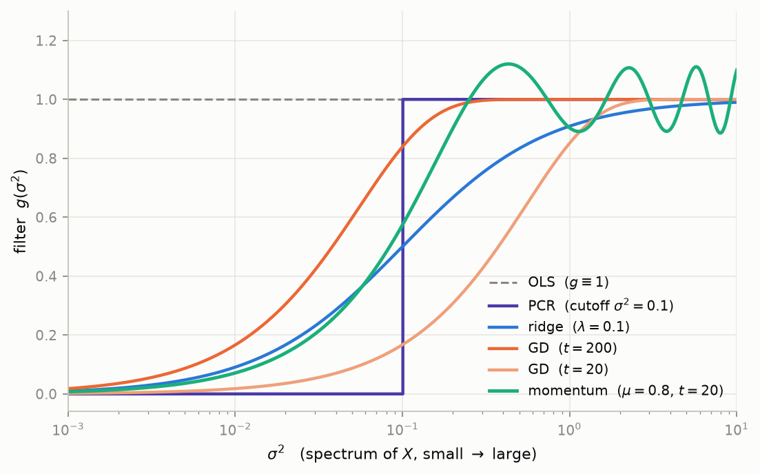
Four of the five curves are doing the same thing: pass the top of the spectrum, suppress the bottom, and differ only in where the knee sits and how abruptly it turns. PCR and Ridge are drawn with the same crossover at $\sigma^2 = 0.1$, which makes the main contrast between them a step versus a smooth ramp. The two GD curves show early stopping sliding along that same family as $t$ grows. While the correspondence with Ridge and GD isn’t exact, there is a very close resemblance when $t=1/(\eta \lambda)$.
Momentum is the one that misbehaves, and it’s worth dwelling on. Its filter overshoots $1$ and oscillates — here it crosses $1$ seven times across the spectrum. Read as an algorithm this is familiar: the heavy-ball iteration is underdamped wherever $(1+\mu-\eta\sigma^2)^2 < 4\mu$, the roots $r_\pm$ go complex, and the residual rings instead of decaying. Read as a statistical estimator it’s much stranger. Plug $g_i > 1$ into the risk decomposition below: the bias term $(1-g_i)^2\theta_i^2$ is nonzero again and the variance term $g_i^2\sigma_\varepsilon^2$ is larger than OLS’s. Both terms are worse. Any direction where the filter sits above $1$ is strictly dominated by simply not shrinking at all: the estimator is paying variance to move away from the target. And because the ripples are non-monotone in $\sigma^2$, two directions with nearly identical singular values can get quite different treatment.
This is one illustration that optimizers designed for faster “numerical” convergence are not always better as statistical estimators when they are used with early stopping. The ML community has known this for some time and is perhaps only recently appreciated in the world of statistics.
The risk breaks apart diagonally
Because everything is diagonal in $U$, so is the risk. Take in-sample prediction risk against the noiseless signal,
\[R(g) = \frac1n\,\mathbb{E}\big\|\hat y - X\beta^\star\big\|^2,\]and project onto the singular directions. Let $\theta_i = u_i^\top X\beta^\star = \sigma_i\,v_i^\top\beta^\star$ be the signal along $u_i$ and $z_i = u_i^\top\varepsilon$ the noise ($\operatorname{Var}(z_i) = \sigma_\varepsilon^2$). Then (appendix)
\[R(g) = \frac1n\sum_i \Big[\underbrace{(1-g(\sigma_i^2))^2\,\theta_i^2}_{\text{bias}^2} + \underbrace{g(\sigma_i^2)^2\,\sigma_\varepsilon^2}_{\text{variance}}\Big].\]The risk is a sum of independent per-direction contributions. In each direction the filter value $g_i \in [0,1]$ trades off exactly two things: a bias term that wants $g_i = 1$ (keep the signal) and a variance term that wants $g_i = 0$ (kill the noise).
Since the directions decouple, the optimal filter minimizes each term on its own:
\[g_i^\star = \frac{\theta_i^2}{\theta_i^2 + \sigma_\varepsilon^2}.\]Keep a direction to the extent its squared signal beats the noise — a per-direction signal-to-noise ratio. This is the Wiener filter. And it has exactly the ridge shape: writing $\theta_i^2 = \sigma_i^2(v_i^\top\beta^\star)^2$, if the signal per unit spectrum $(v_i^\top\beta^\star)^2$ is constant $=\tau^2$ across directions, then
\[g_i^\star = \frac{\sigma_i^2}{\sigma_i^2 + \sigma_\varepsilon^2/\tau^2},\]which is ridge with $\lambda = \sigma_\varepsilon^2/\tau^2$. So Ridge emerges as the optimal linear spectral filter under an isotropic signal model, where the coefficient energy is equal across right-singular directions in expectation.
More food for thought
Many types of (early-stopped) gradient based methods do not fit this mould, like adaptive gradient methods or more classical methods like conjugate gradient. Their iterations depend on $y$ in more complex ways which break the polynomial structure of iterations, making them harder to analyze in a basis. However, these methods would be fascinating to study further. Conjugate gradient is especially interesting: via the Lanczos process it dynamically estimates the spectrum of $X$ as it iterates, which is what gives it fast convergence on clustered spectra. It doesn’t currently use that estimate for anything like shrinkage — but feeding it into an estimated Wiener filter, rather than just using it to accelerate convergence to the unregularized answer, feels like a genuinely open question worth studying.
Once you frame things in terms of $g$, it gives you a palette for making new estimators — e.g. why not “Ridge a Ridge” regression? At the end of the day any of these are reasonable in a sense and just depend on your prior about the Wiener filter: iterating sharpens the knee of the filter independently of where it sits, letting you interpolate between Ridge’s smooth crossover and PCR’s hard cutoff without committing to either extreme. Same question applies to more exotic learning-rate schedules like cosine scheduling — what filter shape does that trace out, and what prior would make it optimal? It’d be interesting to do a larger empirical study of the spectrum of real-world data to see which shapes actually fit.
Lo Gerfo, L., Rosasco, L., Odone, F., De Vito, E., & Verri, A. (2008). Spectral Algorithms for Supervised Learning. Neural Computation, 20(7), 1873–1897.
Yao, Y., Rosasco, L., & Caponnetto, A. (2007). On Early Stopping in Gradient Descent Learning. Constructive Approximation, 26(2), 289–315.
Appendix: derivations
Ridge
Ridge fits $\hat\beta_\lambda = (X^\top X + \lambda I)^{-1}X^\top y$, so $\hat y_\lambda = X\hat\beta_\lambda$. Substitute $X = U\Sigma V^\top$ and $X^\top X = V\Sigma^2 V^\top$; the $V$ factors cancel:
\[\hat y_\lambda = X(X^\top X + \lambda I)^{-1}X^\top y = U\,\frac{\Sigma^2}{\Sigma^2 + \lambda I}\,U^\top y, \qquad g_\lambda(\sigma^2) = \frac{\sigma^2}{\sigma^2 + \lambda}.\]Gradient descent
Run GD on $\tfrac12|y - X\beta|^2$ from $\beta^{(0)} = 0$ with step $\eta$:
\[\beta^{(t+1)} = \beta^{(t)} + \eta X^\top(y - X\beta^{(t)}).\]Map to $\hat y^{(t)} = X\beta^{(t)}$ and work in the $U$ basis. Along $u_i$ the residual is multiplied by $(1 - \eta\sigma_i^2)$ each step, so after $t$ steps the accumulated filter is
\[g_t(\sigma^2) = 1 - (1 - \eta\sigma^2)^{t}.\]For $0 < \eta\sigma^2 < 1$ this climbs from $0$ toward $1$, fastest in the large-$\sigma^2$ directions.
Risk decomposition
With $\hat y = U g(\Sigma^2) U^\top y$ and $y = X\beta^\star + \varepsilon$, orthonormality of $U$ gives a sum over directions. The data along $u_i$ is $u_i^\top y = \theta_i + z_i$; the fit keeps $g_i(\theta_i + z_i)$; the target is $\theta_i$. So
\[R(g) = \frac1n\sum_i \mathbb{E}\big[g_i(\theta_i + z_i) - \theta_i\big]^2.\]Split each error into a deterministic and a mean-zero part:
\[g_i(\theta_i + z_i) - \theta_i = (g_i - 1)\theta_i + g_i z_i.\]The cross term vanishes since $\mathbb{E}[z_i] = 0$, leaving $(1-g_i)^2\theta_i^2 + g_i^2\sigma_\varepsilon^2$ per direction. Minimizing $(1-g_i)^2\theta_i^2 + g_i^2\sigma_\varepsilon^2$ over $g_i$ gives $g_i^\star = \theta_i^2/(\theta_i^2 + \sigma_\varepsilon^2)$.