A Toy Model of the Neural Tangent Kernel
For kernel regression under gradient descent, a little rearranging turns the parameter update into an update on the residuals, and the errors evolve as a linear function of the kernel $K$.1 What got me started on this post was wanting a second equation to sit next to that one: an evolution for $K$ itself, so that the kernel is learned as part of the dynamics rather than fixed up front. I wanted to see what method that implied for different sensible choices.
It turns out the neural tangent kernel already gives you something like this. This post spells out how kernel learning happens in deep linear networks, mostly in the one-hidden-layer case. Linear networks are the smallest setting where the kernel moves at all, which makes them a good place to see what feature learning buys and what it costs.
Gradient Flows in Prediction Space
Take the squared loss $L = \tfrac12\sum_i (f(x_i;\theta) - y_i)^2$ and collect the errors into a vector $e$, with $e_i = f(x_i) - y_i$. To train the model we run gradient descent, $\theta_{k+1} = \theta_k - \eta\,\nabla L(\theta_k)$. Written as $(\theta_{k+1}-\theta_k)/\eta = -\nabla L$ this is a difference quotient, so sending $\eta \to 0$ gives the learning dynamics as a differential equation, $\dot\theta = -\nabla L$, called a gradient flow.
Now let $J$ be the Jacobian of the predictions with respect to the parameters, $J_{i\cdot} = \partial f(x_i)/\partial\theta$. Then $\nabla L = J^\top e$, so the flow is $\dot\theta = -J^\top e$; the chain rule says the predictions move as $\dot f = J\dot\theta$, and the targets do not move at all. Putting those together,
\[\dot e = -K e, \qquad K = JJ^\top.\]The parameters have dropped out. Whatever the model is, the training errors obey a linear differential equation driven by an $n \times n$ matrix built from the Jacobian, and when $f(x_i;\theta)$ is a neural network we call $K$ the neural tangent kernel.
When $f(x;\theta) = \theta^\top x$ is a linear regression, the Jacobian is $X$, so $K = XX^\top$ 2. The kernel is a fact about the data, fixed for the whole of training: the model never learns anything about which inputs are similar, only how to combine them given a similarity it was handed.
The Neural Tangent Kernel
Consider a network with one hidden layer, $f(x) = W_2\,g(W_1x)$. Here the kernel works out to
\[K(x, z) = \sum_{r=1}^m g(w_{1,r}^\top x)\,g(w_{1,r}^\top z) \;+\; (x^\top z)\sum_{r=1}^m w_{2,r}^2\,g'(w_{1,r}^\top x)\,g'(w_{1,r}^\top z).\]The similarity between two inputs now depends on the parameters, so as the weights change over training, so does the kernel. Setting $g(x) = x$ puts us back in the linear case, but with a more interesting kernel than before (since the model is now factored and qualitatively different). Stacking the data into $X$,
\[K = XAX^\top, \qquad A = W_1^\top W_1 + \|W_2\|^2 I.\]The network computes the same linear function that ordinary regression does, and at $A = I$ the kernel reduces to it exactly. What the factoring adds is a weighted Gram matrix, where the weight is low rank plus a multiple of the identity.
Kernel Dynamics
Under gradient flow the two layers obey $\dot W_1 = W_2^\top R$ and $\dot W_2 = RW_1^\top$, with $R = -e^\top X$ the residual correlation. Differentiating $A$ through those gives
\[\dot A = R^\top\beta + \beta^\top R + 2\langle R,\beta\rangle I, \qquad \beta = W_2W_1.\]The evolution of $A$ is driven by the residual, so the kernel stops moving once the network has fit the data. Every term also carries a factor of $\beta$, which means that from a small initialization the kernel barely moves at first: the network has to build the kernel that will go on to train it.
Where it ends up is also explicit. If the weights start balanced, meaning $W_1W_1^\top = W_2^\top W_2$, then gradient flow keeps them balanced, and one can show (appendix) that the kernel converges to
\[A_\infty = (\beta^{*\top}\beta^*)^{1/2} + \|\beta^*\| I,\]where $\beta^*$ is the least-squares solution. The learned term puts mass along the direction the task actually uses, which is what we wanted from a learned kernel. But the identity term does not go away, so the kernel never becomes fully task-dependent. It would be nice to point it more aggressively along the signal, and it turns out depth is what does that. Finally, note that if we define a distance measure $d(x,z)^2 = (x-z)^\top A (x-z)$ part of the distance between two points is dictated by their distance in prediction space.
With the help of GPT (results empirically simulated in the next section), we can ask what $A$ looks like with more depth, $f(x) = W_L\cdots W_1x$, again from a balanced initialization. Write $\beta^* = s\,u^\top$, splitting the solution into its length $s = |\beta^*|$ and its direction $u = \beta^*/|\beta^*|$. Then
\[A_\infty = s^{2(L-1)/L}\left[\,I + (L-1)\,uu^\top\right], \qquad \frac{\lambda_{\max}(A_\infty)}{\lambda_{\min}(A_\infty)} = L.\]Each layer contributes a term of the same size, and all but the first contribute along $u$, so $L-1$ learned terms stack against a single isotropic floor. Depth chips away at the isotropic prior and the kernel gets more pointed in the direction of the signal.
A Simulation
Two-dimensional inputs, one output, mild anisotropy in the data, and a target $\beta^* = (1,1)$ pointing away from either axis, so the direction the data spreads and the direction the task uses are distinguishable. Plain gradient descent on $\beta$ is the $A = I$ baseline.
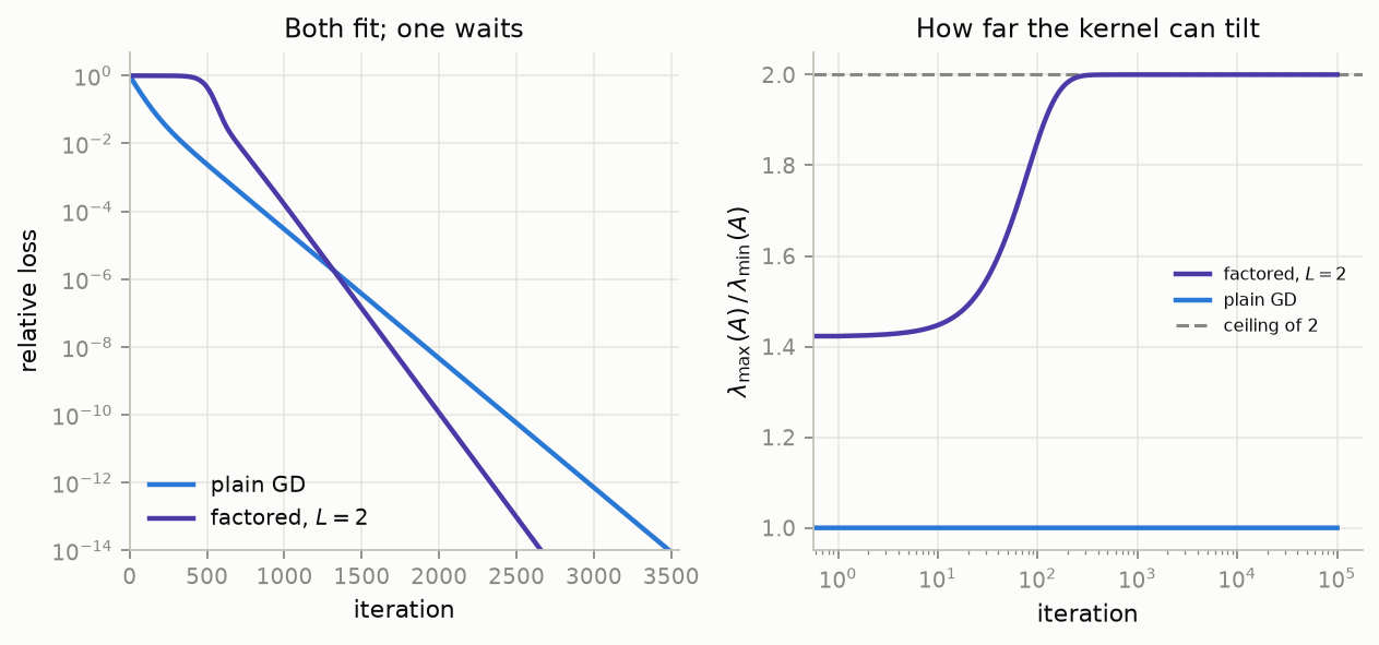
Both learners reach the same fit, but the factored network stalls first: $\beta \approx 0$ makes every term of $\dot A$ small, so there is no kernel to descend along until it has built one. Its anisotropy rises over that same interval and stops flat against the predicted ceiling of $2$, while plain gradient descent sits at $1$ by construction. The curve starts above $1$ because a random $W_1^\top W_1$ is already slightly stretched at initialization; that part is not learned.
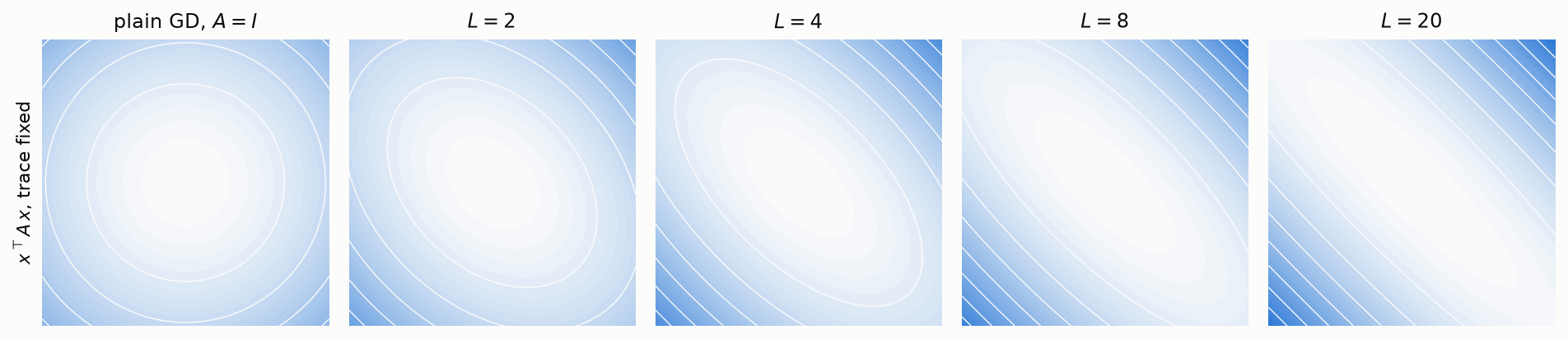
The level sets of $x^\top A_\infty x$ at fixed trace show what the extra depth buys. These read inversely — a contour is narrow along the direction the kernel amplifies — so as depth grows the contour pinches along $\beta^*$, which is the kernel stretching along the signal. Ordinary regression is circular and stays circular. The effect is real but slow, since a factor of $L$ in the eigenvalues is only $\sqrt{L}$ in the distances.
Further Thoughts
The NTK literature is vast and the general results go well past what I have used here. The largest thing I have left out is the distinction between the lazy and feature-learning regimes: for very wide networks the kernel essentially does not move, training reduces to kernel regression with the kernel at initialization, and none of the dynamics above happen at all.
The system of equations is elegant enough that I would like to know how far it bends. What happens to the recursion under layer norm or batch norm, or under normalized gradient methods? Those all change the Jacobian, so they all change the kernel, and it is not obvious in which direction. Finally, it is tempting to turn the whole exercise around: start with interesting dynamics, rather than a loss and an optimization rule, and ask what kind of learning algorithm they imply.
Jacot, Gabriel & Hongler (2018), “Neural Tangent Kernel: Convergence and Generalization in Neural Networks,” NeurIPS.
Saxe, McClelland & Ganguli (2014), “Exact solutions to the nonlinear dynamics of learning in deep linear neural networks,” ICLR.
Arora, Cohen & Hazan (2018), “On the Optimization of Deep Networks: Implicit Acceleration by Overparameterization,” ICML.
Appendix
Gradient flow on $f = W_2W_1x$ conserves $W_1W_1^\top - W_2^\top W_2$, since $\frac{d}{dt}W_1W_1^\top = W_2^\top RW_1^\top + W_1R^\top W_2 = \frac{d}{dt}W_2^\top W_2$. Take the conserved difference to be zero. Then $\beta^\top\beta = W_1^\top W_2^\top W_2W_1 = (W_1^\top W_1)^2$, so $W_1^\top W_1 = (\beta^\top\beta)^{1/2}$, and taking traces gives $|W_2|^2 = \operatorname{tr}(\beta^\top\beta)^{1/2}$, which for a single output is just $|\beta|$. Substituting both into $A = W_1^\top W_1 + |W_2|^2I$ gives the stated form, and $\beta \to \beta^*$ gives $A_\infty$.