Training Dynamics of Bigram Induction
In the post on Transformer Induction Heads we spelled out how a transformer can learn to compute bigrams in a sequence prediction task. This is pretty interesting because from data alone the network learns a computation rather than estimating a parameter. There are a couple follow-up questions I’ve been thinking through: what creates training pressure for this to happen, and when does doing well on training tasks produce a procedure that works well on new ones.
Next-token prediction rewards accurate predictions, not necessarily general algorithms. If a model is trained on a finite set of tasks, the Bayes-optimal predictor under that finite-task distribution performs inference over those specific tasks. This requires memorizing and learning to identify a potentially large set of tasks. A more general algorithm (like learning to compute bigrams) might actually produce worse loss in this case, but can be easier for the network to learn because of architectural limitations or the difficulty of optimization. There is a massive literature on when, how, and why in-context learning develops1. This post is my attempt to think through the tension between learnability and optimality with a couple small simulations.
Setup
We train a small two-layer transformer2 on sequences of 256 tokens drawn from a randomly sampled Markov chain over five states. We draw transition matrices whose rows follow a Dirichlet($\alpha$) distribution. There are two natural ways for the model to use its context (Park, 2025):
- Bigram inference: estimate the transition probabilities from what has followed each token so far. This is what the induction head implements.
- Bigram retrieval: if training uses a finite, fixed pool of chains, recognize which one this is and use its stored transition probabilities.
Inference and retrieval both predict well on training chains, but only inference works on a chain the model has never seen. Training loss can’t tell them apart where it matters, either: cross-entropy only pins down behavior where the training data has mass, and off that distribution the model does whatever its mechanism happens to do.
Payoff: Predictable Sequences Favor Bigrams
When $\alpha$ is small, the rows are peaked (e.g. high probability transitions), so knowing the previous token helps a lot, while larger $\alpha$ leads to more diffuse rows. If we sample a fresh chain for every sequence, nothing can be memorized and the optimal prediction strategy is a smoothed bigram rule3. We can quantify how much a bigram rule buys over just predicting from token frequencies with the expected mutual information between consecutive tokens: $U(\alpha) = \mathbb{E}_P\Big[H(\pi) - \textstyle\sum_i \pi_i\, H(P_i)\Big]$. One might expect this to predict how quickly the transformer learns the bigram mapping since the reward to loss is larger. However, that’s not guaranteed since it says nothing about how easy it is for the network to learn it!
We vary $\alpha$ and track when the induction head forms using an induction score4. Intuitively, an induction head at the current token looks back at what came right after earlier copies of that token; the score is just the fraction of layer 2’s attention that lands on those positions, rescaled so 0 is what uniform attention would get and 1 is a perfect head. It’s worth noting that this doesn’t prove mechanistically we’re doing bigram learning but is strongly suggestive.
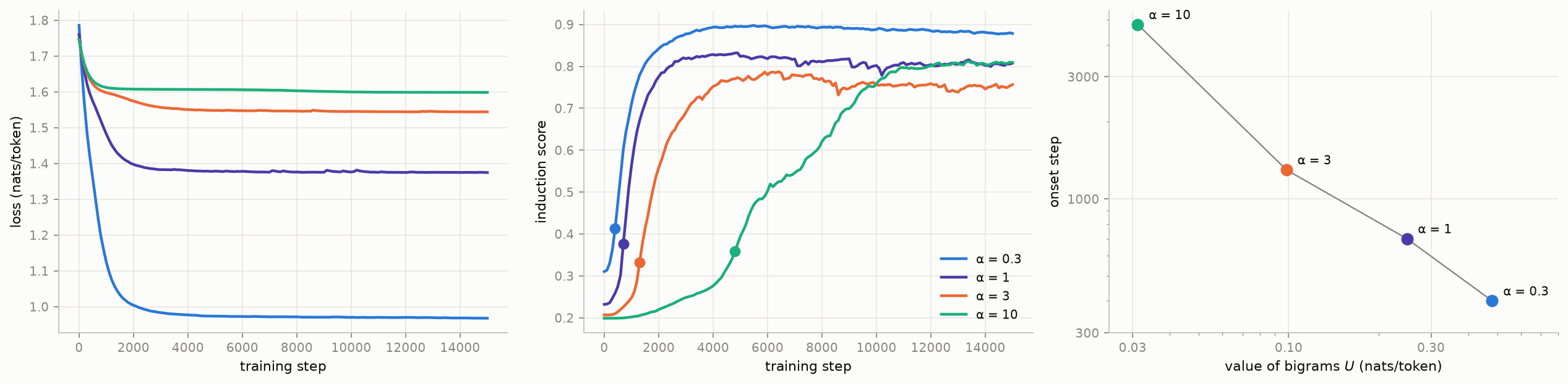
The head forms at step 400 for $\alpha=0.3$, 700 for $\alpha=1$, 1,300 for $\alpha=3$, and 4,800 for $\alpha=10$: a roughly 15-fold drop in payoff gives a 12-fold delay. By step 15k every model is within 0.021 nats of the optimal rule. So even when the architecture nearly hands us the algorithm, it still takes time to find, and that time depends on what it pays. This echoes what’s been seen in language models, which pick up low-order token statistics before higher-order ones, and on one account of scaling acquire skills roughly in order of how much they reduce loss.
Optimality versus Learnability: Finite Pools
This experiment closely follows Park (2025), who show the same transient pattern, where the general rule appears first and is partly displaced by memorization.
In the previous section every sequence came from a freshly sampled chain, so there was nothing to memorize and the bigram rule was optimal. Now we flip that around: we sample a fixed pool of $M$ chains ($\alpha=1$) once, train only on sequences from those chains, and test on chains outside the pool. This is the setting where optimality and learnability can actually come apart, and varying $M$ lets us dial how hard memorizing is. Here the bigram rule is no longer optimal: the best predictor on the training data is a retriever that figures out which of the $M$ chains it’s looking at and uses that chain’s transitions5. It beats the bigram rule at every pool size by a nearly constant margin. Picking out one of $M$ chains takes about $\log_2 M$ bits and is settled within a few dozen tokens, whereas estimating 20 transition probabilities from counts stays noisy for the whole sequence.
| $M$ | Bigram rule on pool chains | Ideal retriever on pool chains | Retrieval advantage |
|---|---|---|---|
| 16 | 1.353 | 1.279 | 0.074 |
| 32 | 1.377 | 1.307 | 0.070 |
| 64 | 1.372 | 1.303 | 0.069 |
| 128 | 1.367 | 1.302 | 0.065 |
| 256 | 1.367 | 1.305 | 0.064 |
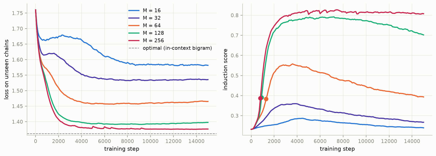
At $M=16$ and $32$ the induction head never forms: the model just memorizes, and loss on unseen chains stays high (1.580 and 1.537 nats, against 1.361 for the optimal rule). At $M=64$ and $128$ the head forms and then partly fades (0.57→0.39 and 0.80→0.70), while training loss pushes past what the bigram rule can achieve (1.357 vs 1.367 at $M=128$). The model finds the general rule first and then trades some of it away for memorization, since that’s what the training loss rewards (see Park 2025). The decline is only partial though, and the score stays well above chance at $M=128$, so the model may well be using both strategies at once. At $M=256$ the head forms and sticks around through 15k steps, and training loss sits right at the bigram level.
Since retrieval pays about the same at every $M$, it isn’t that memorization stops being worth it at $M=256$. My guess is that it just becomes too expensive to reach: each chain only gets about $1/M$ of the gradient signal, and a small model may not have room to store 256 of them anyway. The general rule survives not because it’s optimal, but because it’s what training can find.
Further Thoughts
The two experiments approach learnability from different directions. When there is no competing solution, how quickly the model discovers the general rule depends on how much it improves prediction. When a better-fitting solution is available, the outcome depends on which computation is easier for the model to learn. On a finite pool of tasks, the training objective favors retrieval over generalization, but optimization may still produce the general rule.
It’s tempting to describe inference as Bayesian and retrieval as memorization, but both are posterior predictive strategies under different priors. Bigram inference uses a Dirichlet prior parameterized by a single concentration parameter, while retrieval uses a prior concentrated on the training chains, with their transition matrices stored in the weights. Raventós (2023) find a similar phenomenon in regression: with enough training tasks, transformers behave like ridge regression, which is Bayes-optimal under the Gaussian task distribution rather than the finite training pool. The general solution isn’t the absence of a prior, but a compact representation of one.
These experiments don’t establish what inference the transformer implements internally. They do suggest that what a network learns depends not only on which solution is statistically optimal, but also on which computations are accessible to gradient descent. A generalizable algorithm can emerge even when a more specialized solution achieves lower expected loss, not because the objective rewards generalization, but because the general algorithm is easier to learn.
Edelman, Benjamin L., Ezra Edelman, Surbhi Goel, Eran Malach, and Nikolaos Tsilivis. “The Evolution of Statistical Induction Heads: In-Context Learning Markov Chains.” 2024.
Park, Core Francisco, Ekdeep Singh Lubana, Itamar Pres, and Hidenori Tanaka. “Competition Dynamics Shape Algorithmic Phases of In-Context Learning.” ICLR, 2025.
Raventós, Allan, Mansheej Paul, Feng Chen, and Surya Ganguli. “Pretraining Task Diversity and the Emergence of Non-Bayesian In-Context Learning for Regression.” NeurIPS, 2023.
-
See especially Park (2025) and Edelman (2024) for results very close to the setup we have here. ↩
-
One attention head per layer, width 64, pre-LayerNorm, an MLP after each attention layer (4× width, GELU), learned positional embeddings. Adam (learning rate $10^{-3}$, batch 64), 15k steps, one seed per setting. ↩
-
Each row $P_a$ has an independent Dirichlet($\alpha$) prior. Given the counts $c_{ab}$ of transitions $a\to b$ in the context, the posterior predictive for the token after $a$ is \(p(b \mid a) = \frac{c\_{ab} + \alpha}{\sum\_{b'} c\_{ab'} + k\alpha}.\) ↩
-
Let $A_2[t,s]$ be layer 2’s attention from position $t$ to position $s \le t$. The induction score is $\operatorname{mean}_t \sum_{s \le t:\, x_{s-1} = x_t} A_2[t, s]$, averaged over a fixed held-out batch of 256 sequences. We normalize, $z = (\text{score} - \text{chance}) / (\text{ceiling} - \text{chance})$, and call onset the first step where $z$ stays above 0.25 for 500 steps. The score measures an attention pattern, not a computation: a declining score means layer 2 attends less to positions following earlier copies of the current token, not necessarily that the computation was discarded. ↩
-
With a uniform prior over the pool, the posterior after $x_0, \dots, x_t$ is proportional to $\pi^{(m)}_{x_0} \prod_{s<t} P^{(m)}_{x_s x_{s+1}}$, and the prediction is the posterior-weighted average of the rows $P^{(m)}_{x_t}$. Since it averages over chains instead of committing to one, its loss already includes the cost of being unsure which chain generated the sequence. ↩