Transformer Induction Heads
Introduction
Feed a trained transformer a sequence like ABACABADA and ask what comes after the last A. It answers with a roughly even split over B, C, and D, the tokens that have followed A so far in this prompt. Change the pattern and the answer changes with it. There is no table in the weights it could be reading off, because the answer depends on a string it has never seen. How does it do this?
The answer is that transformers don’t just memorize statistics during training, they learn weights that run an algorithm at inference time. The forward pass isn’t a lookup, it’s a computation. Coming from classical ML, where “learning” means something closer to statistical smoothing, this still feels strange to me.
This post drills into a small transformer to show concretely what that means. We train two-layer attention-only models to do in-context bigram prediction, then take them apart. None of the findings are new: induction heads and the work that followed cover this ground in far more depth (citations at the end). But the existing treatments never quite landed for me: they were either dense tensor algebra (original Anthropic paper), elaborate diagrams, or hand-wavy intuition. This is the version that finally made it click.
Toy Example
Let’s give a quick outline of what has to happen to learn bigrams. Assume we have a sequence like ABACA in our context window and we want the best guess of what comes after the last A. We see that earlier in the sequence we have AB and AC, and so we roughly have the pattern that “when A occurs it’s followed by either a B or a C each with equal probability”. I.e. this is just a rolling bigram calculation. It turns out ICL can implement this.
We’ll stick with a small model that can do the trick: two layers, one attention head each, no MLPs, no layer norm. Rows are positions, so row $i$ of $X \in \mathbb{R}^{n\times d}$ is the residual stream at position $i$, and the whole forward pass is three lines:
\[x_i^{(0)} = t_i + p_i,\] \[A_{ij}^{(\ell)} = \operatorname*{softmax}_{j \le i} \left( x_i^{(\ell-1)} W_{QK}^{(\ell)} \big(x_j^{(\ell-1)}\big)^{\!\top} \right), \qquad x_i^{(\ell)} = x_i^{(\ell-1)} + \sum_{j\le i} A_{ij}^{(\ell)}\, x_j^{(\ell-1)} W_{OV}^{(\ell)},\] \[\text{logits}_i = x_i^{(2)} W_U .\]In order for this to work, the network needs to learn $W_{OV}$ and $W_{QK}$ matrices that implement the following computation. We’ll think of the residual stream as containing a “scratch subspace” where it can read and write intermediate information. We also prepend a sentinel token ^ at position 1, for reasons that will become clear in a moment.
Layer 1: locate the previous token.
The first layer learns to attend to the previous position at every step. Concretely, the layer-1 attention matrix is approximately
\[A_{ij}^{(1)} \approx \mathbb{1}[\,j = i-1\,],\]and $W_{OV}^{(1)}$ copies the token it attends to into the scratch block. After this layer, every position carries both its own token and information about the token immediately before it.
Position 1 is the exception: it has nothing to look back at, so it attends to itself and copies its own token into the scratch block. This is exactly why the sentinel is there. If position 1 held a real token, it would advertise itself in layer 2 as a position preceded by that token, and every later occurrence of that token would spuriously match it. Reserving ^ means position 1 matches nothing.
Layer 2: match and copy.
After layer 1, each position knows both the current token and its predecessor. The second layer uses this to find earlier occurrences of the current token. It queries the token block against the scratch block, so the attention score is $t_i \cdot t_{j-1}$, which is large exactly when the token immediately preceding position $j$ is the current token. The softmax then saturates to a uniform average over all such matches:
\[A_{ij}^{(2)} \approx \frac{\mathbb{1}[\,t_{j-1}=t_i\,]}{|M_i|}, \qquad M_i=\{\,2\le j\le i:\;t_{j-1}=t_i\,\},\]and $W_{OV}^{(2)}$ copies the token at each matching position back into the token block. The resulting contribution to the logits is
\[\frac{1}{|M_i|}\sum_{j\in M_i} t_j,\]which is exactly the empirical distribution of tokens that have previously followed the current one.
Our small example
For ^ABACA, the two attention matrices are shown below. Rows and columns correspond to the six positions, and blank entries are masked by causality:
The last row of $A^{(2)}$ tells the whole story. The final A (position 6) attends equally to positions 3 and 5, whose predecessors are both A. The corresponding tokens are B and C, so the head contributes
to the logits — the equal-probability prediction from the outline above, computed in two attention steps. (The residual stream also carries $t_i$ straight through to the unembedding, so the actual logits include a fixed bonus for repeating the current token; see the appendix.) Rows 2, 3, and 5 illustrate the degenerate case where no previous match exists. In that situation, every score is equal and the attention falls back to a uniform average over the available prefix. Worth flagging now: that fallback is a crude kind of smoothing, and it will come back when we compare against the Bayes-optimal rule.
The construction relies on only two ideas: each attention head can choose where to read from and where to write to, and the attention logits are large enough for both softmaxes to saturate. The explicit $W_{QK}$ and $W_{OV}$ matrices are given in the appendix: everything there is straightforward, just spelled out in detail.
Training a Real Model
Background
We train a two-layer transformer on a synthetic dataset of sampled Markov chains: we generate many sequences of length $L = 100$ from a $K = 3$ state chain whose transition probabilities are sampled uniformly on the simplex. Each sequence gets its own freshly sampled chain, so no particular transition matrix is worth memorizing. This is essentially the setup of Edelman et al. (2024), who study how these heads form over training; here I’m only looking at the trained endpoint.
The model architecture consists of two attention layers, one head each, $d_{\text{model}} = 64$, no MLPs, no layer norm, no biases anywhere — 33,352 parameters in total. We train in batches of 64 across 8,000 steps, so the model sees roughly half a million sequences, a vanishing fraction of the $3^{100}$ possible ones. One small difference from the construction above is that we use relative distances rather than absolute position encodings, because a separate experiment tested generalization to sequences longer than $L$.
Given how the training data was generated the Bayes-optimal predictor has a closed form. Let $n_{vw}$ count the $v \to w$ transitions in the prefix so far and $n_v = \sum_w n_{vw}$ the number of transitions out of $v$. The posterior predictive after seeing current token $t_i = v$ is
\[\Pr(t_{i+1} = w \mid t_{1:i}) = \frac{n_{vw} + 1}{n_v + 3},\]add-one smoothed bigram frequencies. This is the optimal target we will compare against. Note that the idealized construction computes the unsmoothed frequencies, so it cannot be exactly optimal — the gap is largest early in the context, when counts are small.
Results
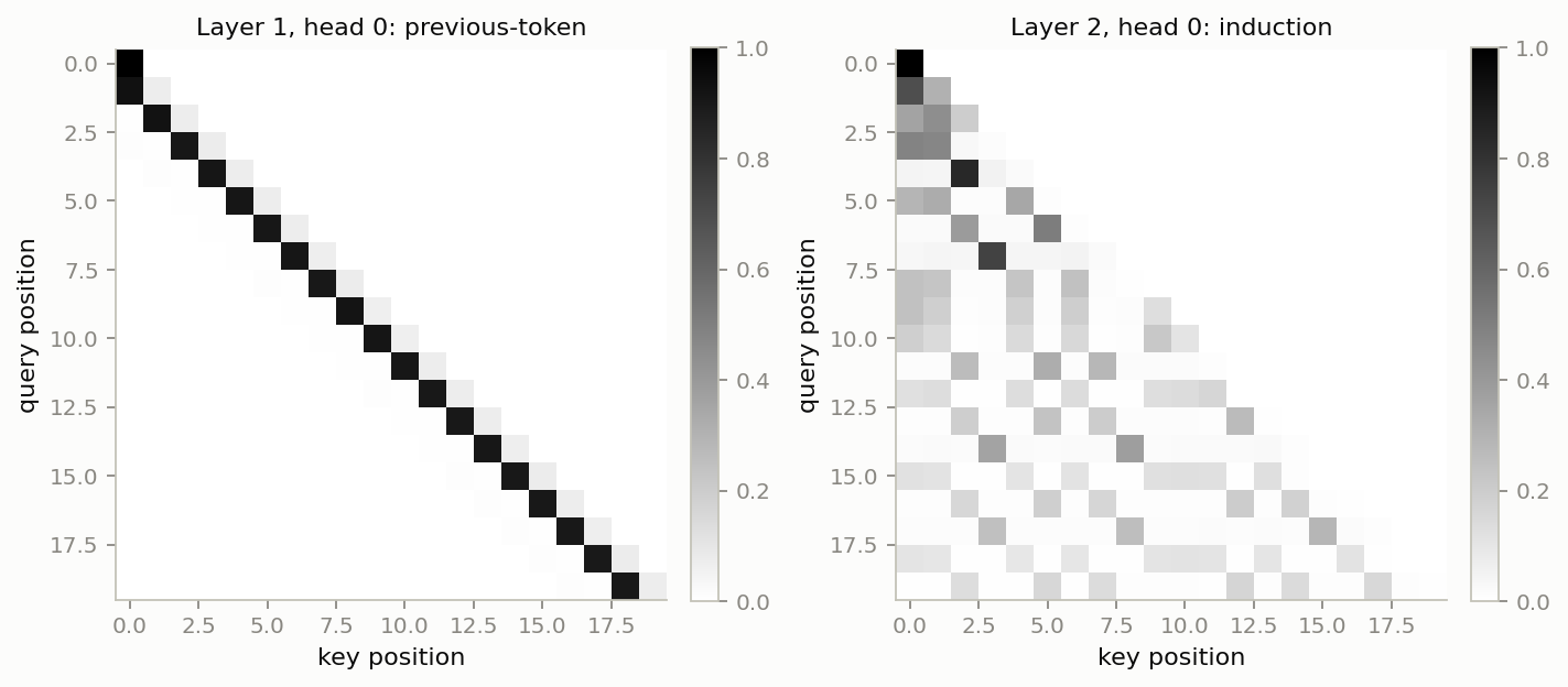
We first show the attention patterns in Layer 1 and Layer 2 for the first segment of an example sequence. It’s easiest to see that Layer 1 is doing what it should: the sub-diagonal pattern shows each position attending to the previous one (with a small shadow of self-attention). In Layer 2 what we should see is each token attending to the positions that followed earlier occurrences of that token — we’ll drill down on this in the next set of plots.
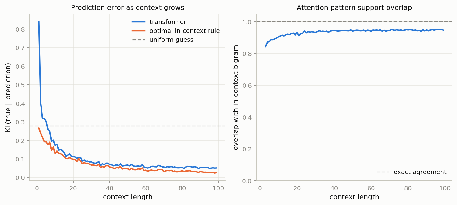
In the plots below we record behavior over a fresh batch of 200 sequences (each of length 100) drawn from freshly sampled Markov chains. The first plot shows the KL divergence from the true next-token distribution, for both the transformer’s estimate and the optimal Bayes rule, at each point in the context. Note that even the optimal rule has non-zero divergence, which decreases as samples accumulate. The transformer and the optimal rule show good concordance after the first dozen tokens.
That concordance is more interesting than it first looks. The clean construction computes raw empirical frequencies, which are badly behaved when a token has been seen once or twice; the Bayes rule smooths them. The trained model tracks the smoothed rule, and the mechanism is visible in the second plot: attention mass does not sit entirely on matching positions, especially early on. The leftover mass spread across non-matching positions is doing roughly what the $+1$ in the numerator does.
The second plot confirms that Layer 2’s attention lines up with the tokens the bigram rule would count, increasingly so as context length grows. The y-axis is the fraction of the head’s attention mass falling on positions that follow an earlier occurrence of the current token. At context length 100, nearly all of it does — a more systematic view than the single example above.
More Food for Thought
The remarkable thing about sequence models is that gradient descent can discover parameters that implement an algorithm. In a task like Markov-chain prediction it is far more efficient to learn a procedure that computes running bigram frequencies from the context than to memorize every sequence one might encounter.
The statistical object I thought I was fitting was an estimator. Mechanistic interpretability suggests a different picture: gradient descent may instead be selecting a computational procedure that, on every forward pass, constructs a new estimator from the prompt itself. There’s a line of work that takes this literally and reads the forward pass as implicit gradient descent (von Oswald et al.); the bigram case here is a much simpler instance of the same idea. If that’s the right way to think about in-context learning, then the questions statisticians ask — consistency, efficiency, robustness, uncertainty — have not disappeared. They have simply moved one level down. The object of study is no longer just an estimator, but a learned algorithm that performs estimation.
Olsson et al., “In-context Learning and Induction Heads,” Transformer Circuits Thread, 2022.
Edelman, Tsilivis, Edelman, Malach & Goel, “The Evolution of Statistical Induction Heads: In-Context Learning Markov Chains,” NeurIPS, 2024.
von Oswald et al., “Transformers Learn In-Context by Gradient Descent,” Proceedings of the 40th International Conference on Machine Learning (ICML), 2023.
Appendix
Explicit matrices for the two-layer construction
This is a constructive example which shows that ICL bigram learning is possible. I got this construction from Anthropic’s Fable model, and it was the first version I saw where all the intuition clicked.
Blocks. Split the residual stream into three blocks of coordinates,
\[\mathbb{R}^d = \underbrace{T}_{|V|} \oplus \underbrace{P}_{n} \oplus \underbrace{B}_{|V|},\]the token block, the position block, and the scratch block. Assume that the token embeddings $t_v = e_v \in T$ and position embeddings $p_i = e_i \in P$ are roughly orthogonal, e.g. one-hot encoding would do this. The vocabulary $V$ includes a sentinel ^, which occupies position 1 of every sequence and is orthogonal to every real token. A vector in the stream is written as a row of blocks $(\,\cdot\,,\,\cdot\,,\,\cdot\,)$, and
The cross-token affinities in the attention head are $s_{ij} = x_i W_{QK} x_j^{\top}$ with a causal mask, so in block form $W_{QK}$ is a $3\times 3$ grid of blocks and the $(a,b)$ block pairs the query’s $a$-block against the key’s $b$-block. Write $\beta$ for the logit scale.
Layer 1 — previous token. Read positions against positions:
\[W_{QK}^{(1)} = \begin{pmatrix} 0 & 0 & 0 \\ 0 & \Omega & 0 \\ 0 & 0 & 0 \end{pmatrix}, \qquad \Omega = \beta \sum_{i=2}^{n} e_i e_{i-1}^{\top},\]so $s_{ij}^{(1)} = \beta\, \mathbb{1}[\,j = i-1\,]$ and the softmax over $j \le i$ puts mass $1 - O(i e^{-\beta})$ on $j = i-1$. Copy $T$ into $B$:
\[W_{OV}^{(1)} = \begin{pmatrix} 0 & 0 & I \\ 0 & 0 & 0 \\ 0 & 0 & 0 \end{pmatrix}, \qquad (t_i, p_i, 0)\, W_{OV}^{(1)} = (0, 0, t_i).\]The head writes $(0,0,t_{i-1})$ at position $i$, and after the residual add
\[x_i^{(1)} = (t_i,\; p_i,\; t_{i-1}).\]Position 1 has nothing to look back at. Its row of $\Omega$ is empty, so all its scores are equal, the softmax over $j \le 1$ puts full mass on itself, and it writes its own token into the scratch block: $x_1^{(1)} = (t_\wedge, p_1, t_\wedge)$. This is the reason for the sentinel. A position whose scratch block holds $t$ advertises itself in layer 2 as “a position preceded by $t$,” so if position 1 held a real token $t_v$, every later occurrence of $t_v$ would match against it and copy $t_v$ into its own logits — inflating the match count and skewing the average. Because $t_\wedge \cdot t_v = 0$ for every real $t_v$, position 1 never matches, and the matching set below can safely start at $j = 2$.
Layer 2 — match and copy. Read the query’s token block against the key’s scratch block — the top-right block, not the bottom-left:
\[W_{QK}^{(2)} = \begin{pmatrix} 0 & 0 & \beta I \\ 0 & 0 & 0 \\ 0 & 0 & 0 \end{pmatrix}, \qquad s_{ij}^{(2)} = x_i^{(1)} W_{QK}^{(2)} \big(x_j^{(1)}\big)^{\top} = \beta\, t_i \cdot t_{j-1}.\]One-hot embeddings make the score exactly $\beta\,\mathbb{1}[\,t_{j-1} = t_i\,]$, so with $m = |M_i|$ matches in $M_i = {2 \le j \le i : t_{j-1} = t_i}$,
\[A_{ij}^{(2)} = \frac{\mathbb{1}[\,j \in M_i\,]}{m} + O\!\big(\tfrac{i}{m} e^{-\beta}\big).\]Copy $T$ back into $T$:
\[W_{OV}^{(2)} = \begin{pmatrix} I & 0 & 0 \\ 0 & 0 & 0 \\ 0 & 0 & 0 \end{pmatrix}, \qquad (t_j, p_j, t_{j-1})\, W_{OV}^{(2)} = (t_j, 0, 0),\]so the head contributes $\big(\frac{1}{m}\sum_{j \in M_i} t_j,\, 0,\, 0\big)$ and
\[x_i^{(2)} = \Big(t_i + \tfrac{1}{m}\textstyle\sum_{j \in M_i} t_j,\;\; p_i,\;\; t_{i-1}\Big).\]Unembedding. Read out the token block, $W_U = \gamma\,(I, 0, 0)^{\top}$:
\[(\text{logits}_i)_v = \gamma\Big(\underbrace{\mathbb{1}[v = t_i]}_{\text{direct path}} + \underbrace{\tfrac{1}{m}\,\#\{j \in M_i : t_j = v\}}_{\text{induction path}}\Big).\]The second term is exactly the in-context bigram distribution: the empirical frequency of $v$ among the tokens that have followed $t_i$ so far. The first is the direct path, a fixed bonus for repeating the current token, which a trained model can cancel through $W_U$ or the layer-2 $OV$ circuit but which the idealized construction leaves in.