Scaling Laws for a Linear Model
Neural scaling laws seek to answer how to best choose model size and the number of training tokens to minimize test loss on a fixed FLOP budget1. Chinchilla’s well known correction was that the large models of the day were badly undertrained and should have been given far more data for the compute they used. These laws get talked about with some mysticism, and they have been used to justify timelines for AI.
I applied the same reasoning to a linear model, where what’s going on is far more transparent. People have done this before with setups different from this one and I don’t claim any of it is new2; the goal is to demystify, and to make very concrete why these can work in a setting we have hope of fully understanding. This is an analogue of the scaling-law calculation, not a model of why transformer scaling exponents take the values they do.
Neural Scaling Laws
This is operationalized by fixing a FLOP budget $C$, choosing a model size $N$, and then training with $D = C/(6N)$ tokens (compute turns out to be well approximated by the product $C \approx 6ND$). The idea is to sweep out FLOP counts and models of various sizes, and the losses closely follow $L(N, D) = E + A N^{-a} + B D^{-b}$ for parameters you can estimate. Minimizing this at fixed $C$ then tells you how to spend the budget,
\[N^* \propto C^{\frac{b}{a+b}}, \qquad D^* \propto C^{\frac{a}{a+b}} .\]Chinchilla found $a$ and $b$ to be roughly equal, so both exponents came out near $1/2$, e.g. scale the model and the data together. That balance is an empirical finding about the fitted exponents, not something the functional form forces. One very important result for large scale transformer training is that across many FLOP scales these follow remarkably coherent power laws, which helps to forecast the performance of large models.
Linear Model Setup
Consider a linear model $y = x^\top\beta^\star + \varepsilon$ with $\operatorname{Var}(\varepsilon) = \sigma_\varepsilon^2$, and defined on a fixed design matrix $X \in \mathbb{R}^{D \times P}$ whose empirical Gram matrix is already diagonalized: $\frac{1}{D}X^\top X = \Lambda = \operatorname{diag}(\lambda_1, \dots, \lambda_P)$. Importantly, here we hold the model size $P$ fixed.
We model the spectrum and signal as:
\[\lambda_k \asymp k^{-\alpha}, \qquad \theta_k^2 \asymp k^{-(2s+1)}, \qquad \theta_k = \sqrt{\lambda_k}\,\beta^\star_k .\]Here $\alpha$ dictates how fast the spectrum decays, e.g. how quickly directions in the data become hard to see, and $s$ says how fast the signal decays along them. Note that power-law spectral and source assumptions like these are standard in this literature. The $\theta_k$ are the prediction coordinates.
Optimization
We consider full batch gradient descent on squared loss initialized at $\beta^{(0)} = 0$. Each step has compute cost $O(DP)$ since we need only a constant number of matrix-vector multiplies, so $C \asymp DT$ where $T$ is the number of rounds of gradient descent. Unlike Chinchilla, gradient descent here touches the data multiple times, and we do not vary parameter count3.
We saw in the Spectral Filtering Post that with full-batch gradient descent in this setup the risk follows
\[R(D, T) = \underbrace{\sum_k \big(1-g_k(T)\big)^2\theta_k^2}_{\text{signal not yet learned}} \;+\; \underbrace{\frac{\sigma_\varepsilon^2}{D}\sum_k g_k(T)^2}_{\text{noise already fit}} .\]where $g_k(T) = 1 - (1-\eta\lambda_k)^T$ and $\eta$ is fixed in the stable range $0 < \eta < 2/\lambda_{\max}$. The idea is that the iterations of GD progressively learn the largest modes in the data first. Training for longer pushes $g_k \to 1$ in more directions, but every direction we learn is also one where we can fit noise, so this is beneficial only up to the bias-variance tradeoff.
The filter turns on for direction $k$ once $\eta\lambda_k T \gtrsim 1$, so after $T$ steps GD has effectively reached $k_T \asymp T^{1/\alpha}$ modes. Everything below sits in the regime $1 \ll k_T \ll P$, e.g. GD has moved past the first few directions but has not yet run out of model. The two terms then become the tail of the signal past $k_T$, and the count of directions learned divided by $D$:
\[R(D, T) \;\asymp\; T^{-2s/\alpha} \;+\; \frac{T^{1/\alpha}}{D} .\]See the appendix for a derivation: the math is nothing more than an exponential approximation and an estimate of a power sum.
Optimization with Fixed Compute
We can write the risk in terms of $T$ and $C$ substituting $D = C/T$, which makes the bias-variance trade-off one-dimensional in the number of gradient steps. It is worth doing this in general, because the specific exponents turn out not to matter much. Suppose the two error sources are any powers of $T$,
\[R(D, T) \asymp T^{-p} + \frac{T^{q}}{D}, \qquad C = DT \qquad\Longrightarrow\qquad R(T, C) \asymp T^{-p} + \frac{T^{q+1}}{C} .\]The first term falls with $T$ and the second rises, so risk is minimized where the two balance, at $T^{p+q+1} \asymp C$. That gives
\[T^*(C) \asymp C^{\frac{1}{p+q+1}}, \qquad D^*(C) \asymp C^{\frac{p+q}{p+q+1}}, \qquad R^*(C) \asymp C^{-\frac{p}{p+q+1}} .\]Two error sources that behave like powers of the training time, a budget that multiplies time by data, and you get power laws out. Compute-optimal scaling laws are what balancing regularly varying error sources against a multiplicative constraint looks like. What is remarkable about neural scaling laws is then not that a power law appears, but that the underlying ingredients stay this stable over many orders of magnitude.
Our case is $p = 2s/\alpha$ and $q = 1/\alpha$, so
\[T^*(C) \asymp C^{\frac{\alpha}{2s+\alpha+1}}, \qquad D^*(C) \asymp C^{\frac{2s+1}{2s+\alpha+1}}, \qquad R^*(C) \asymp C^{-\frac{2s}{2s+\alpha+1}} ,\]and in the simulation in the next section we use $s=1$ and $\alpha = 2$, which gives
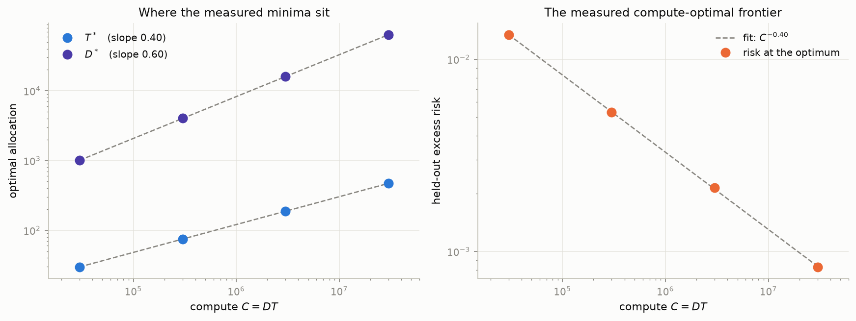
\[T^*(C) \asymp C^{0.4}, \qquad D^*(C) \asymp C^{0.6}, \qquad R^*(C) \asymp C^{-0.4}.\]Note that $\sigma_\varepsilon^2$, the step size $\eta$, and the constants in front of both decay rates move the curves up and down without touching a slope. And what the argument actually needs is not exact pointwise power laws, but power-law asymptotics for the two things that enter it: the number of directions learned by step $T$, and the signal tail left beyond them.
Simulation
Every point on the plots below is a GD run scored on held-out data, against the noiseless signal $x^\top\beta^\star$, so what is plotted is excess risk and the irreducible $\sigma_\varepsilon^2$ never enters. We average over seeds to reduce noise in plots.
We simulate the model above with $\alpha = 2$, $s = 1$, $P = 100$, $\sigma_\varepsilon = 1$ and $\eta = 1$. For each of four compute budgets we sweep $T$, set $D = C/T$, run full-batch GD from zero, and record the risk. Every $D$ therefore needs its own design, so for each one we draw a Gaussian $D \times P$ matrix, orthogonalize its columns, and rescale so that $X^\top X/D = \Lambda$ holds exactly. That design is held fixed while we redraw the observation noise, which makes the derivation’s assumption true rather than approximate and leaves the noise as the only randomness. The minimum of each curve is read off, and the exponents are fit to those minima. (The sweep is centred on a rough guess at $D^*(C)$, so the theory chooses where we look — not what we find there.)
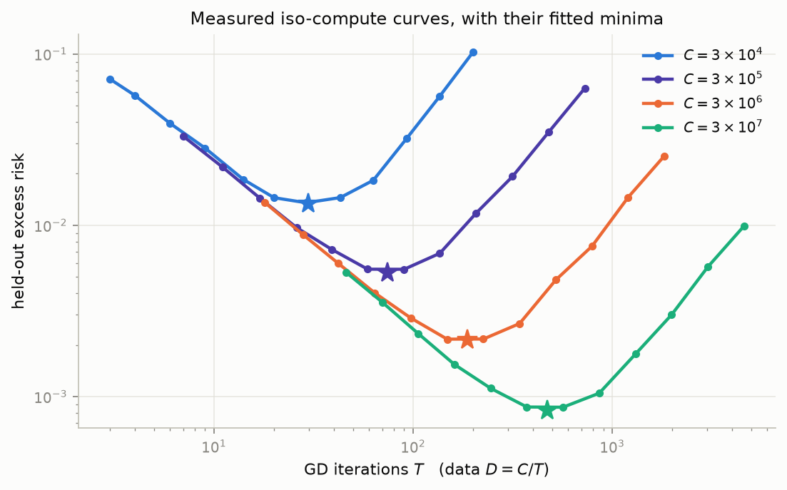
These are the classical analogue of IsoFLOP curves, U-shaped for the reason above: the left branch is undertrained, with signal past $k_T$ never learned; the right branch is data-starved, with $D = C/T$ too small to keep the learned directions from absorbing noise. The minima march right and down as compute grows.
Further Thoughts
Everything above is written in terms of the filter $g$, and nothing forced $g$ to be the one plain gradient descent gives us. Momentum, preconditioning, a learning rate schedule: any of these change $g_k(T)$, and so change the rate and the order in which spectral directions get learned. There is no reason that has to reduce to moving $k_T$ around, but it does move the tradeoff, and it makes the choice of optimizer unusually explicit. We are not only picking something that descends quickly, we are picking which directions get learned per unit of compute, and optimization speed and statistical speed are not the same objective.
The other thread is complexity. What controls the tradeoff here is $k_T$, the number of directions actually learned, which grows during training while $P$ stays fixed. Chinchilla’s $N$ is doing something stranger, since changing it changes what the model can represent, how fast it optimizes, and what a step costs, all at once. Given the balancing argument above, the mystery isn’t that power laws show up. It is that parameter count, a fairly crude proxy for statistical complexity, gives curves as regular as it does.
Worth flagging one difference. The Chinchilla form $L = E + AN^{-a} + BD^{-b}$ is additively separable, so at fixed $D$ it never penalizes a larger model, and its U-curve comes entirely from the budget squeezing $D$. Our variance term $T^{1/\alpha}/D$ couples the two, so at fixed $D$ training longer eventually hurts. That is a limitation of the ansatz rather than a claim about transformers: a separable form cannot express any interaction between $N$ and $D$, so it cannot express overfitting even where overfitting is present.
Appendix
With $\eta$ fixed, $g_k(T) = 1 - (1-\eta\lambda_k)^T \approx 1 - e^{-\eta\lambda_k T}$, which is near $1$ when $\eta\lambda_k T \gg 1$ and near $0$ when $\eta\lambda_k T \ll 1$. The crossover is at $\lambda_k \asymp 1/T$, i.e. at
\[k_T \asymp T^{1/\alpha}.\]Treating the filter as a hard cutoff at $k_T$, the bias term keeps the signal tail,
\[\sum_{k > k_T} k^{-(2s+1)} \asymp k_T^{-2s} = T^{-2s/\alpha},\]and the variance term counts the directions below it, $\sigma_\varepsilon^2 k_T/D \asymp T^{1/\alpha}/D$.
-
Andrej Karpathy has an exceptional note on this https://github.com/karpathy/nanochat/discussions/420 ↩
-
See Lin et al. (2024), “Scaling Laws in Linear Regression: Compute, Parameters, and Data.” for instance. The setup in this note is quite different, however. ↩
-
Longer aside, but parameter count isn’t always a natural measure of statistical complexity. Number of iterations of GD is a nice way to do complexity since it lets us stay in the same model family, e.g. no need to withhold features or use random Fourier bases etc. ↩