What Kind of a Statistician is a Transformer?

In traditional supervised learning we specify the learning algorithm: linear regression minimizes squared error, a decision tree recursively chooses splits. The fitted function changes with the dataset, but the procedure that maps a dataset to that function is known. In-context learning is different: the transformer takes a dataset in its context and produces a fitted function, but the procedure mapping one to the other was itself learned during pretraining. We know how the transformer was trained, but not necessarily what learning rule it learned to execute in context.

This post takes a behavioral approach to that question. Rather than starting with the transformer’s internals, we treat its in-context fit as a statistical estimator and ask what kind of estimator it is. Because the transformer is differentiable, we can directly measure how each observed label influences each prediction. The resulting Jacobian gives us access to a classical statistical toolkit which has historicaly been used to study smoothers, including effective degrees of freedom and Stein’s unbiased risk estimate (SURE).

Jacobian

A trained transformer has fixed weights, but the predictor it implements in context depends on the dataset in its prompt. Let $D=(X,Y)$ be the context dataset and $\hat f_D$ the resulting prediction function, so that for query points $X_q$ we have $\hat Y_q = \hat f_{X,Y}(X_q)$. The transformer defines a learned fitting procedure $D \mapsto \hat f_D$. Holding $X$ and $X_q$ fixed, we can ask how that fitted function responds to perturbations of the observed labels. Define

\[J = \frac{\partial \hat Y_q}{\partial Y}, \qquad J_{ij} = \frac{\partial \hat f_D(x_{q,i})}{\partial y_j},\]

so $J_{ij}$ says how much the prediction at $x_{q,i}$ moves when we perturb $y_j$.

This has exactly the shape of an object statisticians already have vocabulary for. A large part of classical nonparametrics concerns estimators of the form $\hat y = Sy$ where $S$ is a smoother matrix: kernel regression, splines, ridge, $k$-NN, etc. If our in-context learner were exactly such an estimator, its Jacobian with respect to $y$ would simply be $S$.

In general $J$ is only a local linearization, but that is already enough to ask which observations drive which predictions and to measure quantities like effective degrees of freedom. If the map happens to be affine in $Y$, then $J$ stops being merely local and becomes the smoother matrix itself. More generally, for differentiable estimators the Jacobian unlocks an estimate of prediction risk we will study in a later section.

Setup

We want a problem simple enough that we know what the optimal learning rule should be. Each sequence draws a fresh function $f(x)=\phi(x)\cdot w$, with $w\sim N(0,I)$ and $\phi$ the first $P=5$ Legendre polynomials on $[-1,1]$. We then draw $n=64$ pairs with $x_i\sim U[-1,1]$ and $y_i=f(x_i)+0.1\epsilon_i.$. A fresh $f$ every sequence means nothing is memorizable across sequences: whatever the model does at test time, it has to do in context.

The useful feature of this prior is that the Bayes rule is known exactly. It is a linear smoother,

\[S = \Phi_q(\Phi_c^\top\Phi_c+\sigma^2I)^{-1}\Phi_c^\top,\]

whose effective degrees of freedom have a hard ceiling $\operatorname{tr}(S)\to P=5$ (derivation in the appendix). So we have a concrete optimal estimator to compare against: five degrees of freedom because the underlying function class has five dimensions. The models are small pre-LN causal decoders, width 64 with 4 heads and no positional embeddings, trained for 20k steps at depths 1, 2, 4, and 8. See the appendix for more training details.

Learning a Smoother

The Jacobian is, in principle, only a local description of the model. The first question is how much of the actual fit it captures.

We sample 32 prompts from the data-generating process and compare the transformer’s in-context predictions against the affine approximation $Jy+b$, where $b$ is the model’s prediction at $y=0$.

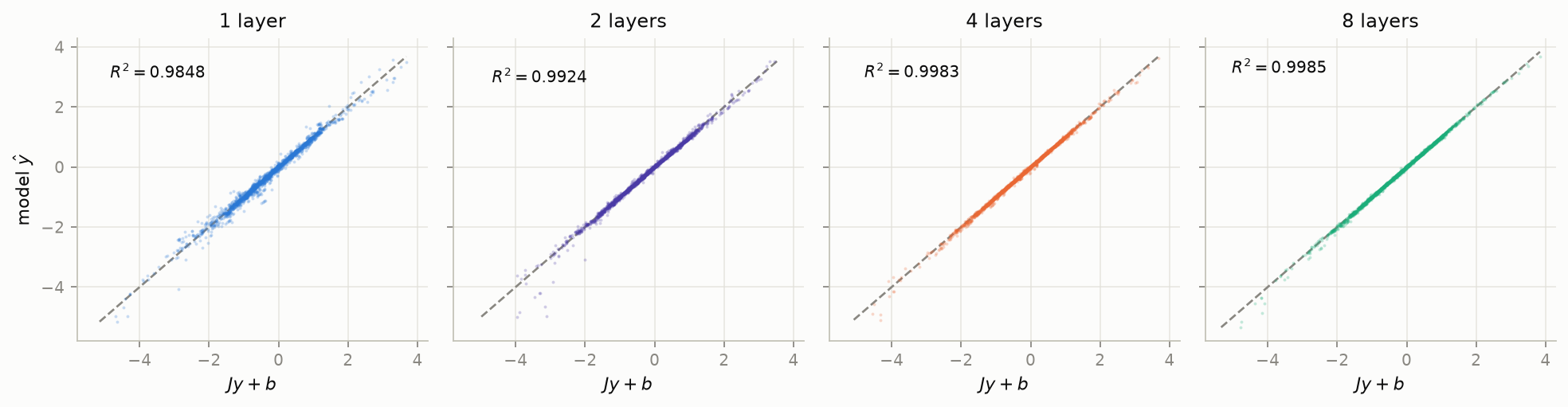
The agreement is extremely close, and $b$ is small. So on this problem the Jacobian is doing considerably more than giving a useful local approximation: the transformer’s learned fitting rule is very nearly a linear smoother in the observed labels, $\hat y\approx Jy$.

That lets us ask what smoother it learned. Below we plot $J$ as a heatmap for a single prompt across the four depths, alongside the Bayes smoother. The lower row takes a slice through each kernel at the origin, showing which context points a prediction at $x_q\approx0$ actually draws on.

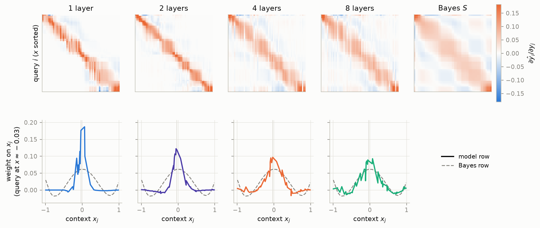
Every model has learned something local, but the shallow models are much more local than the Bayes rule. As depth increases, the kernel becomes more diffuse: predictions pool information across a broader region of the context. We can make that difference precise by looking at the effective degrees of freedom of the learned smoother.

More Capacity, Fewer Degrees of Freedom

The effective degrees of freedom of a differentiable estimator can be measured by how sensitive its fitted values are to the observed labels,

\[\operatorname{df}(\hat y)=\sum_i \frac{\partial \hat y_i}{\partial y_i}=\operatorname{tr}(J).\]

For a linear smoother $\hat y=Sy$, this reduces to the familiar $\operatorname{tr}(S)$. This quantity appears in the classical bias-variance accounting for smoothers, and the same quantity appears in Mallows’ $C_p$, GCV, and SURE. For an ordinary linear model it reduces to the number of fitted parameters.

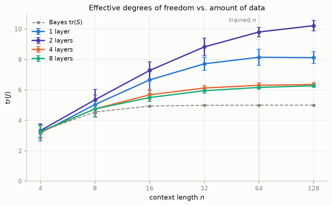
For the transformer we can compute $\operatorname{tr}(J)$ directly¹. Large $\operatorname{tr}(J)$ means a more flexible fit; small $\operatorname{tr}(J)$ means more shrinkage and pooling. Our models were trained on contexts of length 64, but at test time we can vary how much data they receive and watch the learned estimator change. With only a few points in context, the models keep their effective degrees of freedom small. As more data arrives, they support more complexity and $\operatorname{tr}(J)$ rises. The surprising part is the ordering across depths: the shallower models run at higher effective degrees of freedom than the deeper ones.

The naive expectation might run the other way, since depth buys capacity and capacity sounds like complexity. But the capacity of the network and the complexity of the fitted function are different things. Here, depth appears to buy the ability to pool information across the context rather than lean heavily on the nearest few observations. The depth-8 model spends its additional capacity implementing something closer to the Bayes rule, and the Bayes rule is a simpler estimator in this sense. More network capacity produces fewer effective degrees of freedom.

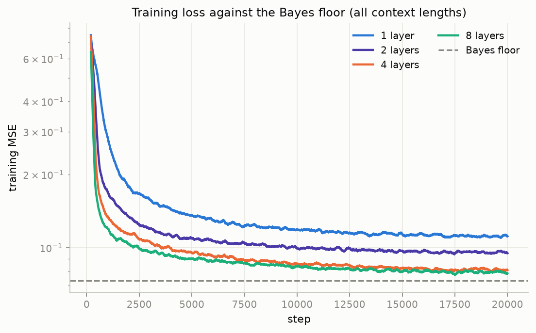
The training curves in the appendix suggest this ordering is not an artifact of where training stopped.

Risk Estimates

So far we have taken advantage of an empirical fact particular to this problem: the transformer is nearly linear in the observed labels. But the same Jacobian also gives us useful statistical quantities when that is not true. Under Gaussian noise, Stein’s unbiased risk estimate is

\[R_{\mathrm{SURE}} = \frac{1}{n}\|\hat y-y\|^2-\sigma^2+\frac{2\sigma^2}{n}\operatorname{tr}(J).\]

The first term is the error we can observe on the noisy data. The $\operatorname{tr}(J)$ term corrects for the optimism introduced by fitting to those same observations, giving an unbiased estimate of prediction risk. The important point for us is that SURE does not require $\hat y$ to be linear in $y$. It only requires a differentiable map from the observed labels to the fitted values. A transformer gives us exactly that, and autograd gives us the derivatives. Assuming the noise level is known or can be estimated, we can therefore estimate the risk of the in-context fit without knowing the learning algorithm the transformer is implementing.

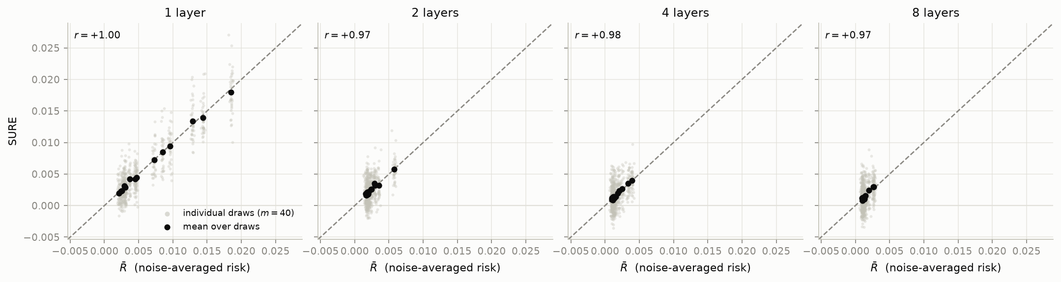
The plot below shows the distinction directly. We sample 16 problems and, for each one, draw 40 realizations of the noise (SURE is computed on training examples)². Each black dot is the average SURE for one problem and sits close to that problem’s true noise-averaged risk. The grey points are individual noise draws. Their spread is the reminder that SURE is unbiased but still noisy: any single estimate can be well off. This tool is bread-and-butter for statistical machine learning but less well known in the AI community.

From Statistics Back to Mechanism

The data-generating process here was deliberately simple, and it is not surprising that a sufficiently deep model gets close to the optimal estimator. The point was to start in a setting where we know what should happen and check whether these tools recover it. The machinery itself is more general: any differentiable in-context learner defines a map from observed data to fitted values, and the same tools let us probe the estimator it has learned.

The natural next step is to connect this statistical description back to mechanism. If we trained across a range of noise levels, would the transformer learn to infer the noise level from context and adjust its shrinkage accordingly? More broadly, I’d like to know whether these models rediscover the statistical toolkit we already know works: shrinkage, ensembling, etc. and how those procedures are implemented mechanistically³. Tabular foundation models seem like a particularly promising place to ask what kind of statisticians these models have learned to be.

Garg, Shivam, Dimitris Tsipras, Percy Liang, and Gregory Valiant. “What Can Transformers Learn In-Context? A Case Study of Simple Function Classes.” NeurIPS, 2022.

Akyürek, Ekin, Dale Schuurmans, Jacob Andreas, Tengyu Ma, and Denny Zhou. “What Learning Algorithm Is In-Context Learning? Investigations with Linear Models.” ICLR, 2023.

Han, Chi, Ziqi Wang, Han Zhao, and Heng Ji. “Explaining Emergent In-Context Learning as Kernel Regression.” 2023.

Appendix

A. The Bayes Smoother

Let $\Phi_c$ be the $n\times P$ feature matrix for the context points, with row $i$ given by $\phi(x_i)^\top$, and let $\Phi_q$ be the corresponding matrix for the query points. Under the prior $w\sim N(0,I_P)$ and observation model $y=\Phi_cw+\sigma\epsilon,$ the posterior mean prediction is

\[\hat y_q=\underbrace{\Phi_q(\Phi_c^\top\Phi_c+\sigma^2I)^{-1}\Phi_c^\top}_{S}y.\]

So the Bayes estimator is exactly linear in the observed labels, with smoother matrix $S$.

For in-sample prediction, $\Phi_q=\Phi_c$. Since the features are normalized so that $\mathbb E[\phi(x)\phi(x)^\top]=I/P$, for large $n$ we have $\Phi_c^\top\Phi_c\approx(n/P)I$. Hence

\[\operatorname{tr}(S)\approx P\frac{n/P}{n/P+\sigma^2}\to P=5.\]

Thus the Bayes estimator has at most five effective degrees of freedom, reflecting the five-dimensional function class.

B. Training Curves

Training loss (200-step moving average) against the Bayes floor of 0.0732 for the same objective. Nothing is still descending appreciably at 20k steps, so the final losses are converged and the ordering is not an artifact of where training stopped.

1. Computing a full Jacobian requires a backward pass through the model per output dimension, but if we are only interested in its trace we can approximate it more cheaply via Hutchinson’s trace estimator. It is also worth noting that because forward passes tend to be cheap, transformer-based ICL functions are particularly amenable to leave-one-out analysis. ↩

2. Queries are appended after the full context, so every query attends to all $n$ labels. ↩

3. One story is that certain types of tabular foundation models perform amortized Bayesian inference, but I haven’t seen a convincing mechanistic accounting for this. ↩