Epoch-wise double descent in OLS
I was initially a bit skeptical of double descent in the OLS regression setting. In the usual exposition one plots test error against the number of predictors and gets the second descent right at the $p=n$ interpolation threshold. That always felt like a bit of a sleight of hand: once $p>n$, you have to specify which interpolating solution you’re talking about. In practice this means baking in an inductive bias, such as the minimum-norm solution. As it happens, many of the optimization algorithms we already use—gradient descent, for example—produce exactly this bias.
Gradient descent (GD) on OLS feels like a cleaner comparison. The model class is fixed throughout training, and only the amount of optimization changes. If the x-axis in the bias-variance tradeoff is meant to represent “complexity,” then the number of GD iterations is a natural candidate: each step reduces training error and progressively removes bias.
This post looks at double descent through that lens. The surprising part is that the phenomenon survives even when “complexity” is measured by optimization time rather than model size. In the end, the picture becomes quite simple: gradient descent turns on the spectrum one eigendirection at a time, and double descent is just what happens when those directions alternate between carrying more signal than noise and less. What looks mysterious in parameter space becomes almost inevitable in spectral coordinates.
Setup
Fix a design matrix $X \in \mathbb{R}^{n\times p}$ and write its SVD as
\[X = \sqrt{n}\,U\,\Lambda^{1/2}V^\top, \qquad U^\top U = I_p,\qquad \Lambda = \operatorname{diag}(\lambda_1 \ge \dots \ge \lambda_p),\]so the empirical second moment is exactly
\[\hat\Sigma \;=\; \frac{X^\top X}{n} \;=\; V\Lambda V^\top \;=:\; \Sigma .\]Here, $V$ is a fixed rotation, meaning $X$ has correlated, non-orthogonal columns—nothing is diagonal in the coordinate basis. Data and test points are defined as:
\[y = Xw^* + \varepsilon,\quad \varepsilon\sim\mathcal N(0,\sigma^2 I_n), \qquad x_{\text{test}} \sim \mathcal N(0,\Sigma).\]Risk. Excess squared error on a fresh point is
\[R(w) \;=\; \mathbb E_x\big(x^\top w - x^\top w^*\big)^2 \;=\; (w-w^*)^\top\Sigma\,(w-w^*) \;=\; \lVert w-w^*\rVert_\Sigma^2 .\]The $\Sigma$ subscript captures the entire difference between prediction risk and estimation error. Since $\Sigma = V\Lambda V^\top$, it is diagonalized in the eigenbasis ${v_i}$. Writing $d_i = v_i^\top(w-w^*)$, we get $R(w)=\sum_i \lambda_i d_i^2$. That is the sole structural fact used below.
Gradient descent has a closed form
Performing GD on the objective $L(w)=\frac{1}{2n}\lVert Xw-y\rVert^2$ starting from $w_0=0$ with step size $\eta$:
\[w_{t+1} \;=\; w_t - \eta\big(\Sigma w_t - X^\top y/n\big).\]Projecting onto $v_i$, and letting $a_i := v_i^\top w^*$ and $g_i := v_i^\top X^\top\varepsilon/n$, the coordinates decouple completely:
\[v_i^\top w_t \;=\; f_i(t)\Big[a_i + \frac{g_i}{\lambda_i}\Big], \qquad \boxed{\,f_i(t) = 1-(1-\eta\lambda_i)^t\,}\]The term $f_i$ acts as a low-pass filter over the spectrum: mode $i$ turns on at $t \sim 1/(\eta\lambda_i)$. Stability requires $\eta < 2/\lambda_{\max}$. (Equivalently, GD at step $t$ behaves like ridge regression with an effective regularization $\lambda_{\text{eff}}\sim 1/(\eta t)$.)
The risk, in two pieces
Since $\mathbb E[g_i]=0$ and $\mathbb E[g_i^2]=\sigma^2\lambda_i/n$, a bit of algebra lets us split the risk into bias and variance:
\[R(t) \;=\; \underbrace{\sum_i \lambda_i a_i^2\,(1-f_i)^2}_{\text{bias},\ \downarrow} \;+\; \underbrace{\frac{\sigma^2}{n}\sum_i f_i^2}_{\text{variance},\ \uparrow}\]Defining the signal energy of a mode and the noise price as:
\[s_i := \lambda_i a_i^2, \qquad c := \frac{\sigma^2}{n}, \qquad\text{we can rewrite}\qquad R(t) = \sum_i\Big[s_i(1-f_i)^2 + c\,f_i^2\Big].\]At the extremes:
\[R(0) = \sum_i s_i, \qquad R(\infty) = \frac{p\,\sigma^2}{n}.\]Both pieces are monotone in $t$. Therefore, the shape of the risk curve is determined entirely by the order in which the modes switch on.
As the number of training rounds increases, the filter $f_i$ approaches 1 for modes ordered from largest to smallest eigenvalues. As each mode turns on, the risk shifts from signal energy $s_i$ to noise price $c$, producing a net change of:
\[\Delta_i \;=\; c - s_i \;=\; \frac{\sigma^2}{n} - \lambda_i a_i^2 .\]Therefore, $R(t)$ is simply a running cumulative sum of $\Delta_i$ walked down the spectrum. Double descent is nothing more than traversing regions of the spectrum where the signal energy alternates between exceeding and falling below the noise price. In other words, each eigendirection is either worth learning ($s_i > c$) or not ($s_i < c$). Gradient descent simply decides when each of those bets gets placed.
A minimal example
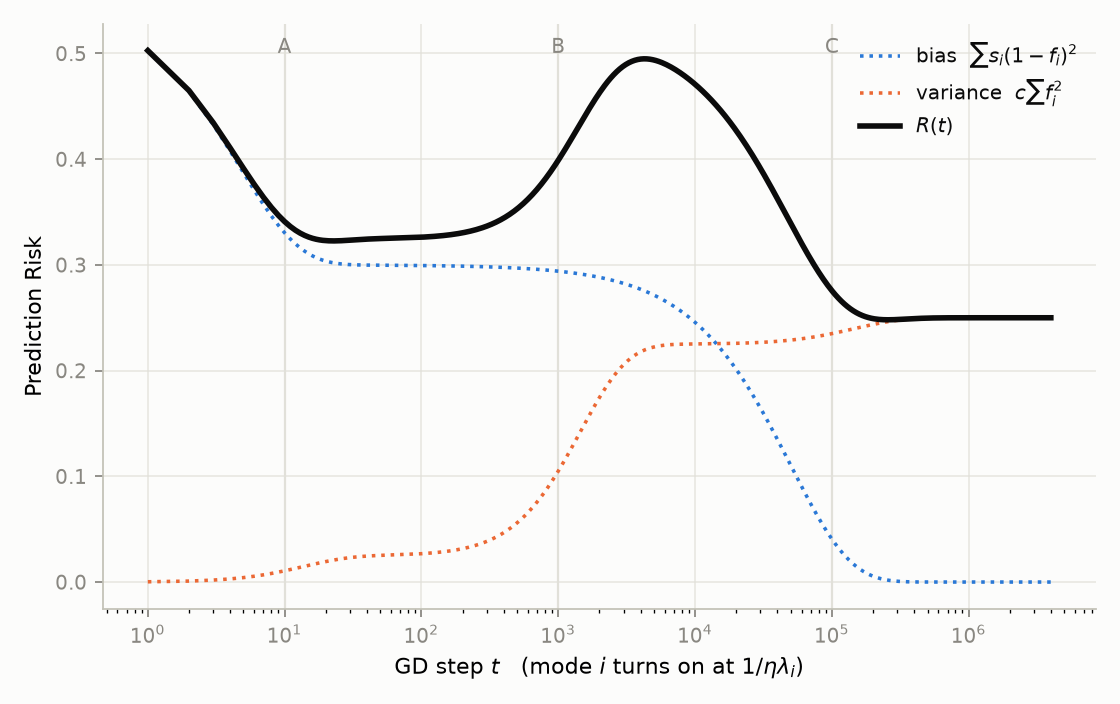
To see this numerically, we can construct an example where the spectrum is divided into three distinct regions (A, B, and C):
- Block A: Clear, fast signal.
- Block B: Pure noise—400 directions with zero signal, representing pure noise-fitting.
- Block C: A slow direction carrying a large coefficient ($a^2 = 60$), separated by eigenvalue ratios of $100\times$ to prevent phase overlap.
Using three blocks with $n = 2000$, $\sigma^2 = 1$, and $c = 5\times10^{-4}$:
| block | $k$ | $\lambda$ | $a^2$ | $s=\lambda a^2$ | $s/c$ | $\sum\Delta$ | turns on |
|---|---|---|---|---|---|---|---|
| A | 50 | $1$ | $0.005$ | $10c$ | $10$ | $-0.225$ | $t\approx 10$ |
| B | 400 | $10^{-2}$ | $0$ | $0$ | $0$ | $+0.200$ | $t\approx 10^{3}$ |
| C | 50 | $10^{-4}$ | $60$ | $12c$ | $12$ | $-0.275$ | $t\approx 10^{5}$ |
Individually, bias and variance behave exactly as expected: more rounds of GD reduce bias and increase variance. However, their interaction creates a funky double-descent shape.
Some extra food for thought
Modern statistical learning increasingly treats the optimizer as a first-class citizen. Especially in overparameterized settings—or whenever early stopping is used—the optimizer is not merely a computational tool, it is part of the estimator itself.
In spectral coordinates this becomes almost unavoidable. OLS, Ridge, PCR, early-stopped gradient descent, momentum methods, and many other algorithms are all spectral estimators: they differ only in the filters they apply across the eigenspectrum. Which estimator is “best” therefore depends not on some abstract notion of complexity, but on how the signal is distributed over that spectrum.
Thinking this way also changes how I view the bias-variance tradeoff. Complexity is not just about reducing bias. Different optimization procedures reveal different spectral modes at different rates, and the resulting risk depends on whether those modes carry signal or only noise. From that perspective, double descent is not a mysterious exception to the classical story—it is simply one of the natural behaviors that emerge when learning unfolds spectrally